MySQL Window Functions Part 2

First introduced as part of the SQ:2003 Standard and available in MySQL 8.0, window functions in MySQL are compelling, but the syntax can also be a little intimidating when you first start using them. This post is the second in a series where we will discuss window functions – including breaking down the syntax and using examples of different window functions. All the code examples in this post use the database table and data we created in Part 1.
As we progress through these examples, we should remember that most (if not all) of this functionality can be handled with any programming language. However, I prefer to let the database do what it does best - retrieve and manipulate data.
LAG() and LEAD() Example
Two window functions that are very closely related allow us to look at a row of data n rows before or n rows after the current row. These are LAG() and LEAD() respectively.
If we want to show the sum of the points for the current player and the previous and next players, we would use this query:
SELECT `full_name`,
       `group_name`,
       RANK() OVER( PARTITION BY `group_name`
          ORDER BY `points` DESC
          ) group_rank,
      `points`,

       `points` +
       LAG( `points`, 1, `points` ) OVER ( PARTITION BY `group_name`
          ORDER BY `points` DESC
          ) with_player_above,

      `points` +
      LEAD( `points`, 1, `points` ) OVER ( PARTITION BY `group_name`
         ORDER BY `points` DESC
         ) with_player_below

FROM `player`
ORDER BY group_name, group_rank;
As you can see, each of these functions takes three arguments:
- The column we wish to retrieve.
- The number of rows we wish to offset. In our example, we want to look at one row before and one after our current row, so we pass a value of
1. - The default value to return if the result of the function call is
NULL. The default value can be a hardcoded value or column name.
In each row of the result set, we add the value returned from LAG() and LEAD() to the current value of the points column in the current row.
This image shows the results of the above query.
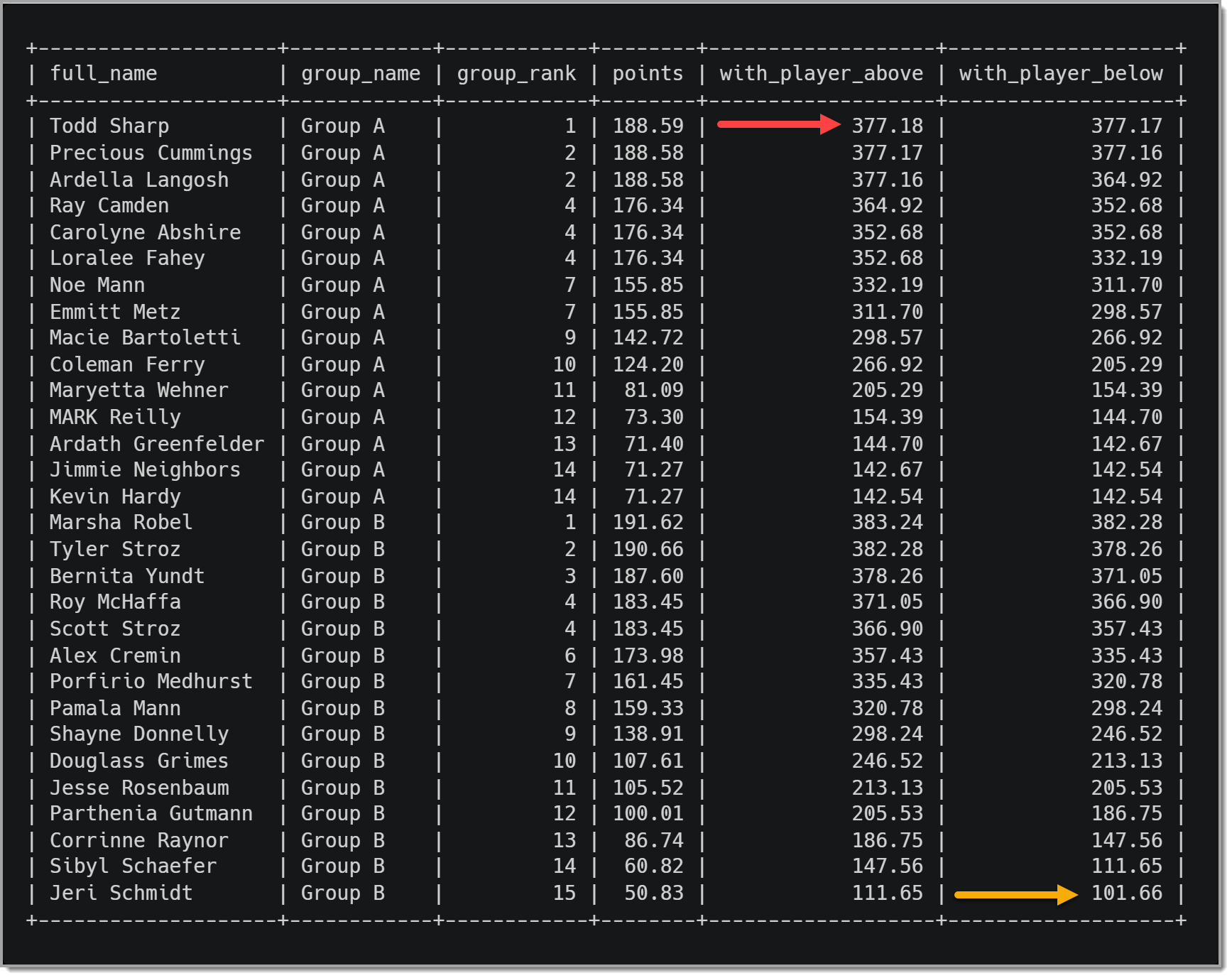
The results of our calls to LAG() and LEAD() indicated by the red and yellow arrows may be interesting. If we omitted the third argument (the default value is the result is NULL), each result would be NULL. Since we are returning the value of points in the current row if the result was NULL, each of these is the value of points doubled.
NTILE() Example
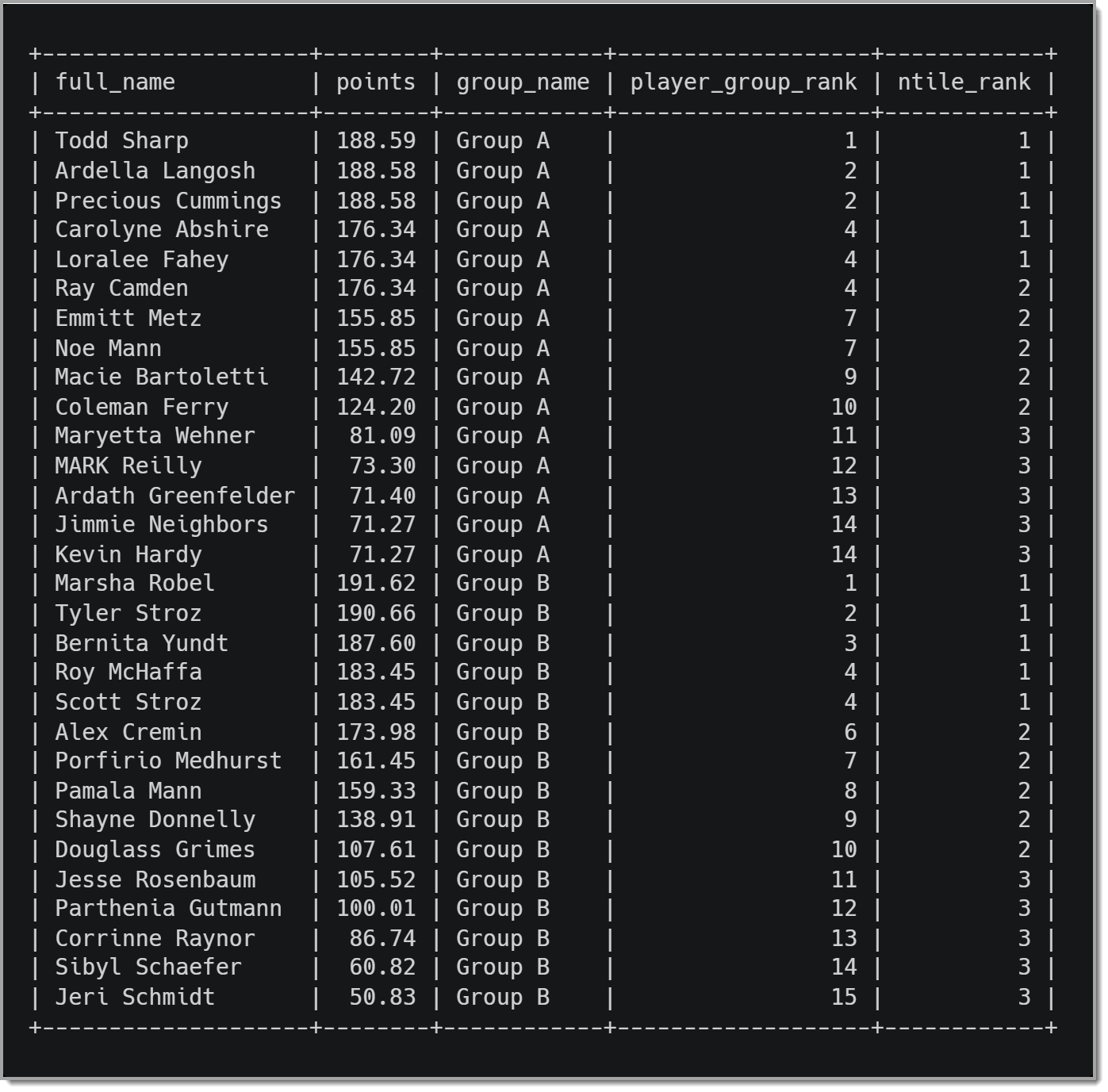
Let’s assume that we need to separate the players into three groups within each of our groups based on their total points. This sub-grouping allows us to see what players are in their group’s top, middle, and bottom third.
To accomplish this, we use the NTILE() function.
SELECT `full_name`,
   `points`,
   `group_name`,
   RANK() OVER( PARTITION BY `group_name`
      ORDER BY `points` DESC
      ) player_group_rank,
   NTILE(3) OVER ( PARTITION BY `group_name`
       ORDER BY `points` DESC, `full_name`
       ) ntile_rank
FROM `player`
ORDER BY group_name, player_group_rank, full_name;
We pass in a single argument to NTILE(), the number of groups into which we would like to break our data. In our example, we use 3 because we want to see the players broken up into three groups.
When we run this query, we see results that look like this:
PERCENT_RANK() Example
In more extensive data sets, it might be helpful to see the percentile rank of each row of data. PERCENT_RANK() will calculate the percentage of players with more points than the current player.
We can return that information using the query below:
SELECT `full_name`,
   `points`,
   `group_name`,
   RANK() OVER( PARTITION BY `group_name`
      ORDER BY `points` DESC
   ) player_group_rank,
   ROUND(
      PERCENT_RANK() OVER ( PARTITION BY `group_name`
         ORDER BY `points` DESC
   ) * 100 ,2 ) pct_rank
FROM `player`
ORDER BY group_name, player_group_rank, full_name;
PERCENT_RANK() does not take any arguments, and to make the information easier to read, we are multiplying the result by 100 and then rounding to 2 decimal places.
The results of this query can be seen in the image below.
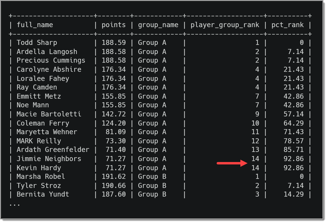
The interesting thing to note in the result set is that there is no score where 100% of the other scores are higher in Group A. This happens because Jimmie Neighbors and Kevin Hardy are tied for last place in the group.
Using SUM() as a Window Function
As I noted in Part 1 of this series, some aggregate functions can be used as window functions if we add an OVER() clause. So let’s take a look at how we can do that.
If we wanted to show what percentage of the total group points a given player’s points equals. To accomplish this, we could use the query below:
SELECT `full_name`,
   `points`,
   `group_name`,
   RANK() OVER( PARTITION BY `group_name`
      ORDER BY `points` DESC
   ) player_group_rank,
   ROUND(
      (points / SUM(points) OVER ( PARTITION BY `group_name`) * 100), 4
   ) point_pct
FROM `player`
ORDER BY group_name, player_group_rank, full_name;
Notice how we add an OVER() clause to SUM(), partitioning the data by the group name. The value returned from this call to SUM() will return the total number of points for each player in the group. To determine what percentage the given player is of the total points, we divide the player’s points by the result of the call to SUM() and multiply by 100. We then round that value to 4 decimal places.
The results of this query would look similar to the picture below.
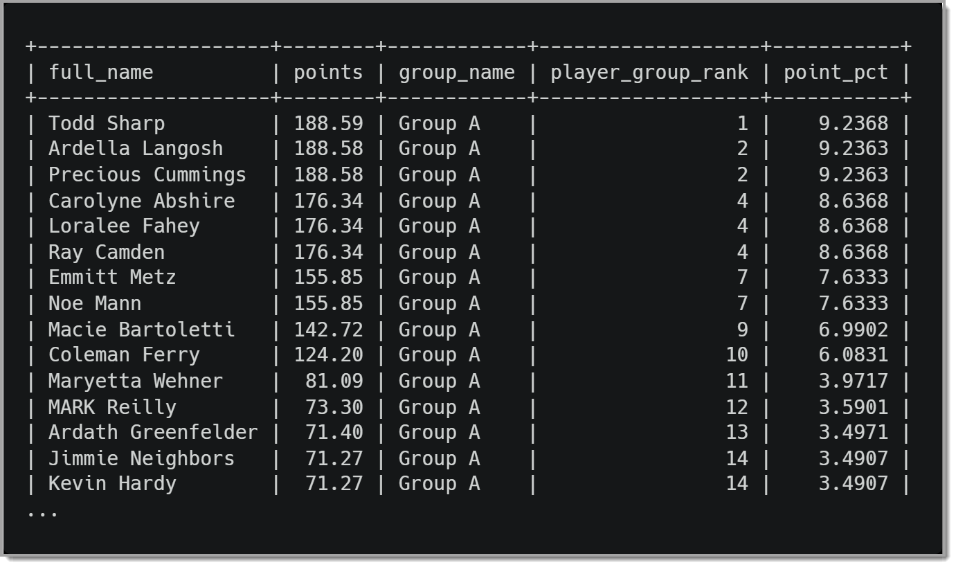
The results show that of the 15 players in Group A, Todd Sharp contributed 9.2368% of the points. In case you are wondering, I purposely rounded these values to four decimal places so we could see the difference between the top two player percentages in Group A.
For more information on using other aggregate functions as window functions, check out the MySQl documentation.
Using window frames
When we use a PARTITION BY clause in a window function, we tell MySQL how we want to group the data. With window functions, we can get even more granular in what set of data we want to return. A frame clause provides this granularity.
When dealing with a frame clause, we can limit the data used for a particular window function. Using a frame clause, we define a range of what rows to include in our subset of data. For example, in this definition, we use the following to set the boundaries of our frame:
UNBOUNDED PRECEDING- every row in the partition that precedes the current rowUNBOUNDED FOLLOWING- every row in the partition that follows the current rown PRECEDING- n number of rows preceding the current row.n FOLLOWING- n number of rows following the current row.CURRENT ROW- the current row.
When specifying a range, we use starting and ending points. If there is no range defined, the default range is as follows:
- The entire partition is used if there is no
ORDER BYclause in the window function. - If an
ORDER BYclause is present in the window function, the range isBETWEEN UNBOUNDED PRECEDING AND CURRENT ROW.
ROWS Example
When using a frame clause, they can be defined in two different ways. First, ROWS determines how many rows to include. For example, if we only want to use the two rows preceding the current row, we could use ROWS 2 PRECEDING in our definition. We will use RANGE in our definition if we want to use the value to determine how many rows to use. For example, if we want to limit the frame to be players within ten points, we would use RANGE 10 FOLLOWING.
An example of using ROWS is calculating a running total returned with each player. The query for this would be:
SELECT `full_name`,
       `points`,
       `group_name`,
       RANK() OVER( PARTITION BY `group_name`
          ORDER BY `points` DESC
          ) player_group_rank,
      SUM( points ) OVER ( PARTITION BY `group_name`
          ORDER BY `points` DESC
          ROWS UNBOUNDED PRECEDING
          ) running_total
FROM `player`
ORDER BY group_name, player_group_rank;
Note that we are only using the starting point for the window frame. In this case, the endpoint is CURRENT ROW. Our call to SUM() is adding the points in the current row and every preceding row in the partition.
The results for this query would resemble the image below.
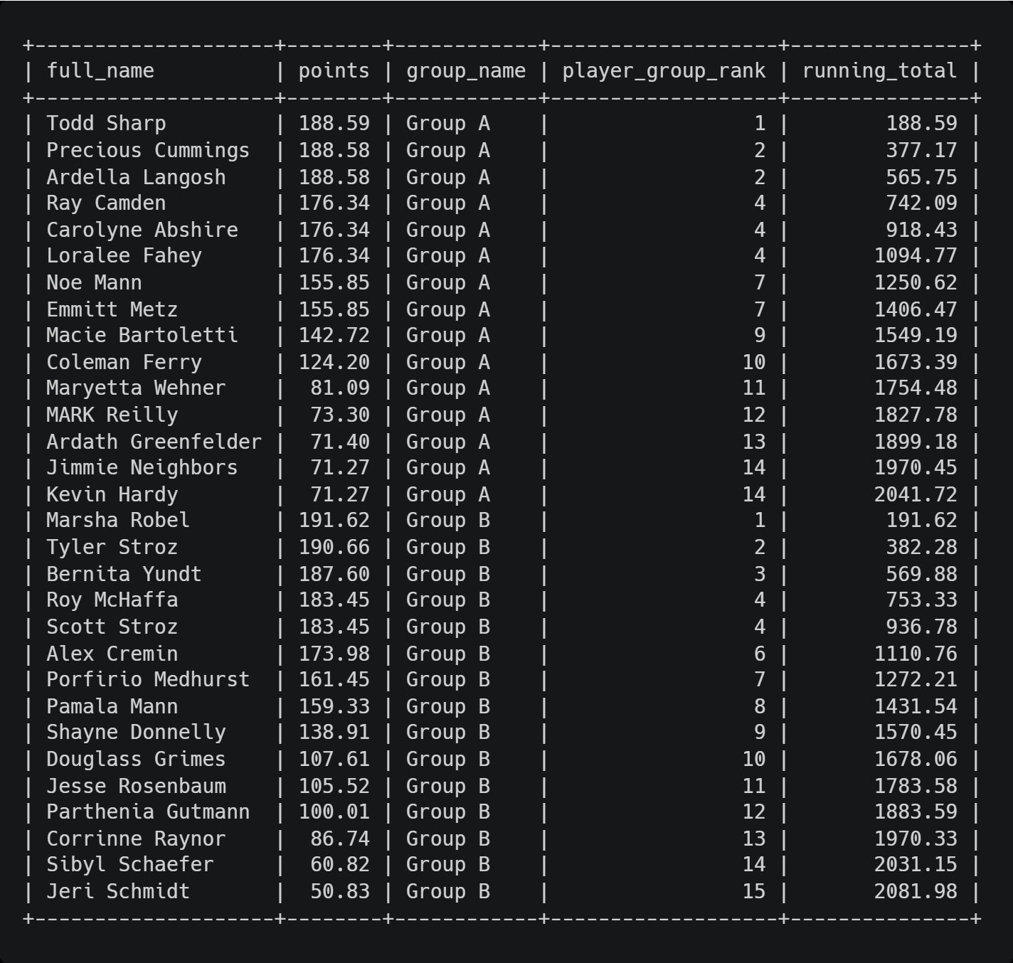
The image above shows that the running total restarts when a new group starts. So if we wanted to do a running total for all players, we would remove the partition in our call to SUM().
RANGE Example
Using ROWS as part of a window frame is straightforward. RANGE, however, is a bit more involved. When we use RANGE, we pull all rows where the value matches the criteria. We could use a different number of rows in the window function for each row in the result set.
Below is a query that will return how many players are ten or fewer points behind the current player.
SELECT `full_name`,
       `points`,
       `group_name`,
       RANK() OVER( PARTITION BY `group_name`
          ORDER BY `points` DESC
          ) player_group_rank,
       COUNT( * ) OVER ( PARTITION BY `group_name`
          ORDER BY `points` DESC
          RANGE BETWEEN CURRENT ROW AND 10 FOLLOWING
          ) - 1 within_ten_points
FROM `player`
ORDER BY group_name, player_group_rank;
We use COUNT() as a window function in this example. If you look at the window frame, you can see our range is the points value of the current row to any row within 10 points of that value. We subtract one from the result because that range definition will include the current row, and we do not want to include the current player in our count.
The results of this query will look like the following:
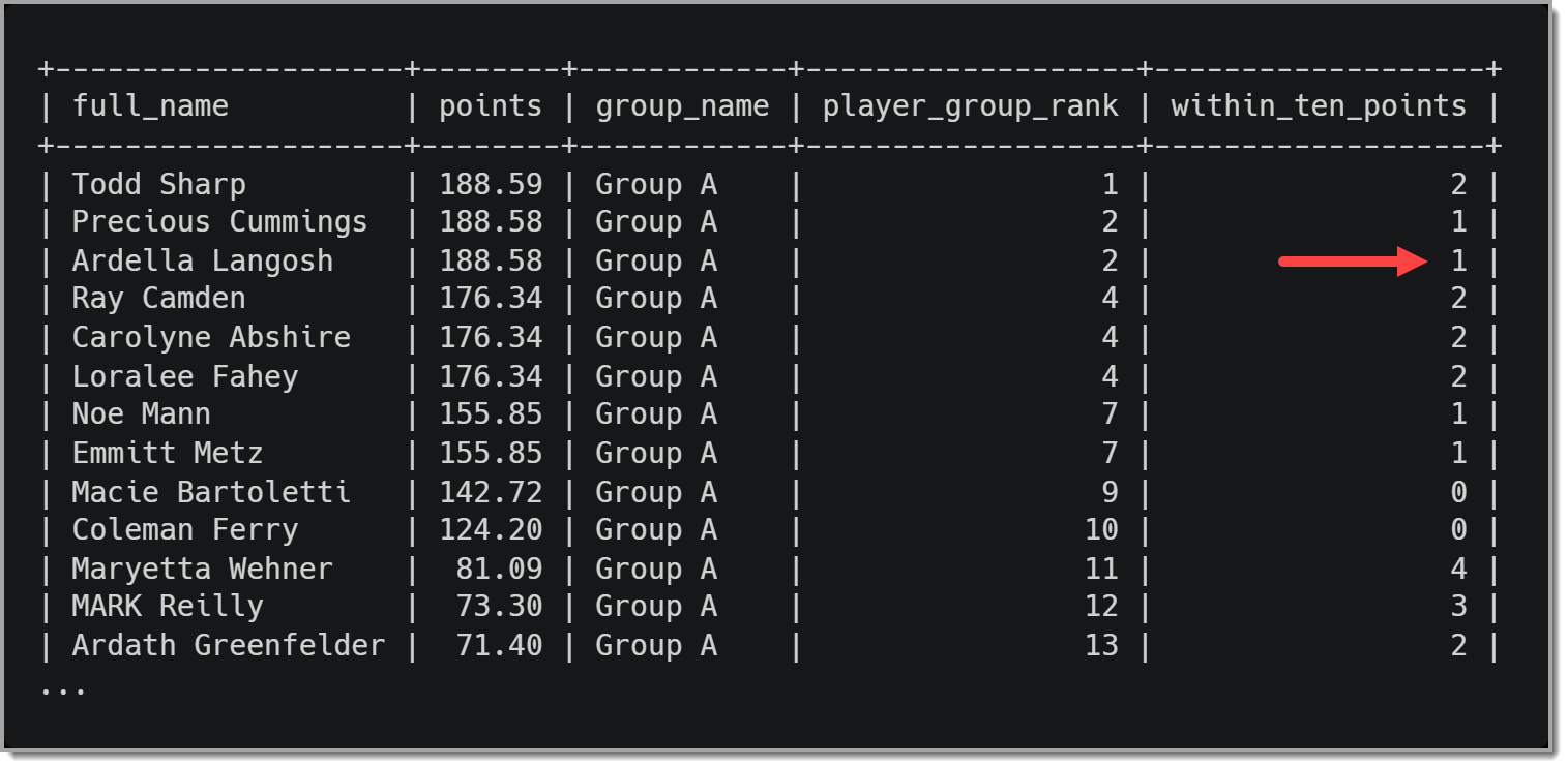
An interesting bit is that Ardella shows one player is within ten points, but the player below her in the standings is more than ten points behind. This is because Ardella and Precious Cummings are tied, so the points for Precious are used in this calculation.
It is important to note that we can only use RANGE for values in the ORDER BY that are numbers or dates. So, for example, we could not use RANGE if the ORDER BY clause in the COUNT() was using full_name.
Wrap Up
While the functionality of window functions can be replicated in any programming language, using them to return data directly from the database can make the developers’ job a bit easier. The syntax of window functions can be a bit daunting, but breaking it down into individual parts can make it easier to read and understand. I hope this series will make it easier for you to handle that breakdown.
Check out the documentation to learn more about window functions.
Photo by Waldemar Brandt.
