MySQL Window Functions Part 1

First introduced as part of the SQ:2003 Standard and available in MySQL 8.0, window functions in MySQL are compelling, but the syntax can also be a little intimidating when you first start using them. This post is the first in a series where we will discuss window functions – including breaking down the syntax and using examples of different window functions.
Definition
Before we can break down the different parts of window functions, let’s define what they are and what they do. Window functions are built-in MySQL functions that offer aggregate-like functionality on a defined range of rows in a query. While other aggregate functions, such as SUM(), will group the result into a single row or grouped rows, window functions will return a value for every row in a query result. Window functions can be aggregate functions, such as SUM(), or non-aggregate functions, such as RANK(). In this post, we will show examples of some non-aggregate window functions.
Setting Up Our Data
Before we go any further, let’s get our demo data set up. Here are the scripts we will use to define and populate the table for this post. This data represents a fictional competition where players earn points during each match. The information we use shows the total number of points a player has accumulated.
-- Create the schema
CREATE SCHEMA IF NOT EXISTS `window-function-demo`;
-- Switch to use the schema
USE `window-function-demo`;
-- Drop table
DROP TABLE IF EXISTS `player`;
-- Create the table
CREATE TABLE IF NOT EXISTS `player` (
`id` INT NOT NULL AUTO_INCREMENT,
`full_name` VARCHAR(45) NOT NULL,
`points` DECIMAL(5,2) NOT NULL,
`group_name` VARCHAR(10),
PRIMARY KEY (`id`)
);
As you can see, this table has just four columns: an id that is the primary key, the name of the player, the number of points scored by the player, and the group to which the player belongs.
 -- Insert data
insert into player (full_name, points, group_name) values ('Noe Mann', 155.85, 'Group A');
insert into player (full_name, points, group_name) values ('Precious Cummings', 188.58, 'Group A');
insert into player (full_name, points, group_name) values ('Maryetta Wehner', 81.09, 'Group A');
insert into player (full_name, points, group_name) values ('Todd Sharp', 188.59, 'Group A');
insert into player (full_name, points, group_name) values ('Macie Bartoletti', 142.72, 'Group A');
insert into player (full_name, points, group_name) values ('Emmitt Metz', 155.85, 'Group A');
insert into player (full_name, points, group_name) values ('Ardella Langosh', 188.58, 'Group A');
insert into player (full_name, points, group_name) values ('MARK Reilly', 73.3, 'Group A');
insert into player (full_name, points, group_name) values ('Ardath Greenfelder', 71.4, 'Group A');
insert into player (full_name, points, group_name) values ('Coleman Ferry', 124.2, 'Group A');
insert into player (full_name, points, group_name) values ('Ray Camden', 176.34, 'Group A');
insert into player (full_name, points, group_name) values ('Carolyne Abshire', 176.34, 'Group A');
insert into player (full_name, points, group_name) values ('Jimmie Neighbors', 71.27, 'Group A');
insert into player (full_name, points, group_name) values ('Kevin Hardy', 71.27, 'Group A');
insert into player (full_name, points, group_name) values ('Loralee Fahey', 176.34, 'Group A');
insert into player (full_name, points, group_name) values ('Corrinne Raynor', 86.74, 'Group B');
insert into player (full_name, points, group_name) values ('Parthenia Gutmann', 100.01, 'Group B');
insert into player (full_name, points, group_name) values ('Porfirio Medhurst', 161.45, 'Group B');
insert into player (full_name, points, group_name) values ('Alex Cremin', 173.98, 'Group B');
insert into player (full_name, points, group_name) values ('Sibyl Schaefer', 60.82, 'Group B');
insert into player (full_name, points, group_name) values ('Marsha Robel', 191.62, 'Group B');
insert into player (full_name, points, group_name) values ('Shayne Donnelly', 138.91, 'Group B');
insert into player (full_name, points, group_name) values ('Tyler Stroz', 190.66, 'Group B');
insert into player (full_name, points, group_name) values ('Douglass Grimes', 107.61, 'Group B');
insert into player (full_name, points, group_name) values ('Jesse Rosenbaum', 105.52, 'Group B');
insert into player (full_name, points, group_name) values ('Jeri Schmidt', 50.83, 'Group B');
insert into player (full_name, points, group_name) values ('Roy McHaffa', 183.45, 'Group B');
insert into player (full_name, points, group_name) values ('Scott Stroz', 183.45, 'Group B');
insert into player (full_name, points, group_name) values ('Pamala Mann', 159.33, 'Group B');
insert into player (full_name, points, group_name) values ('Bernita Yundt', 187.6, 'Group B');
Window Function Syntax
Using RANK(), DENSE_RANK() and OVER()
Window functions have several clauses, but all have the OVER() clause in common. Non-aggregate window functions require an OVER() clause, while aggregate functions will work like window functions when we add one. For example, if we wanted to display the rank of each player based on the number of points they scored, we would use the RANK() window function, and the query would look like this:
SELECT `full_name`,
`points`,
RANK() OVER(
ORDER BY `points` desc
) player_overall_rank,
`group_name`
FROM `player`
ORDER BY player_overall_rank;
As you can see, one part of the OVER() clause is an ORDER BY clause. So, in this example, we are telling RANK() to return the rank value based on the descending order of points.
The results of this query show the rank of each player would look like this:
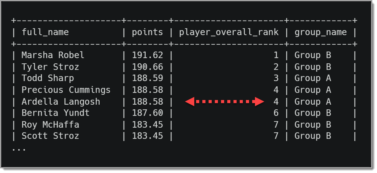
Notice that the rank value is sequential until it gets to Ardella Langosh, and four repeats. This repetition is because Ardella and Precious Cummings have the same number of points, each ranking 4th overall. Also, the next player, Bernita Yundt, is ranked 6th. This action is due to the fact we used RANK(), where it will skip numbers if more than one value is the same as another. This logic is consistent with how leaderboards for competitions often work.
As long as we have access to the data that we use as a tiebreaker, we can use this to show only one player per rank. In our case, we will use the player’s name as the tiebreaker, so if two or more teams are tied, the player whose name comes first alphabetically will be ranked higher.
The query to enforce this tiebreaker would be:
SELECT `full_name`,
       `points`,
       RANK() OVER(
          ORDER BY `points` desc, full_name
          ) player_overall_rank,
       `group_name`
FROM `player`
ORDER BY player_overall_rank;
Notice that we added full_name to the ORDER BY in the RANK() window function.
The results of this query would appear as:
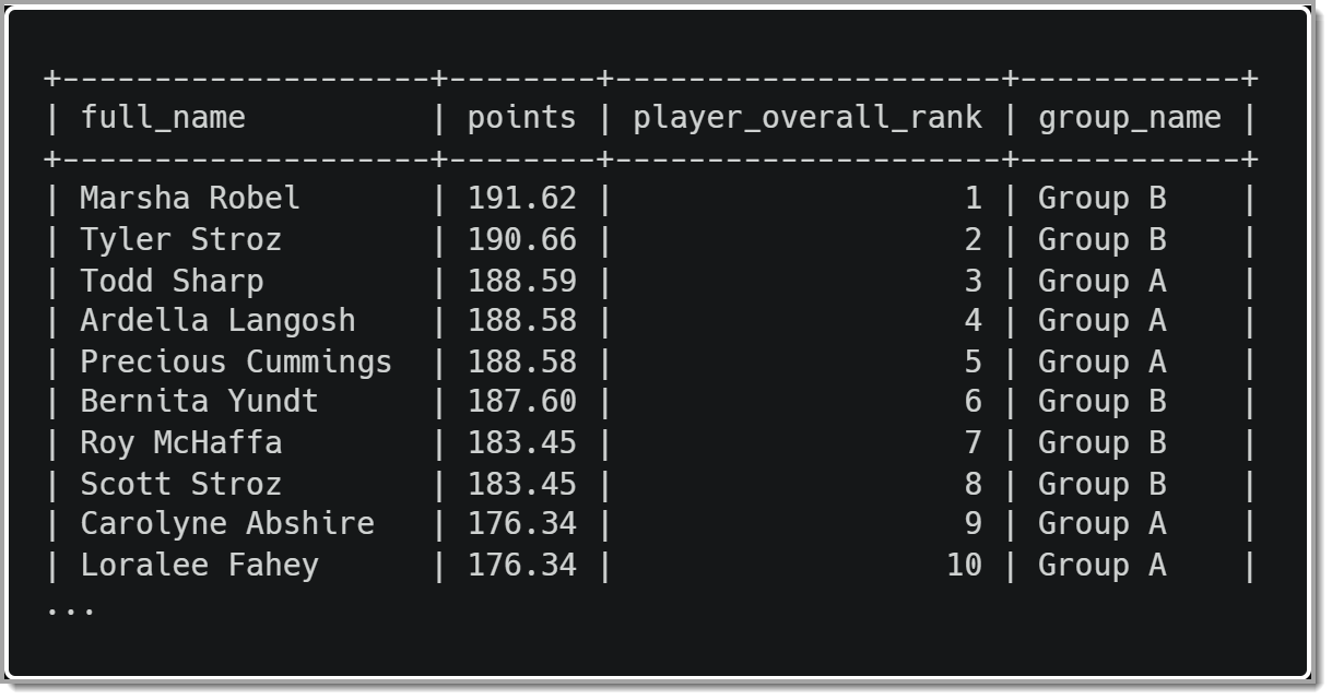
As we can see, each player is now ranked 1-10 instead of duplicating ranks among players with the same score.
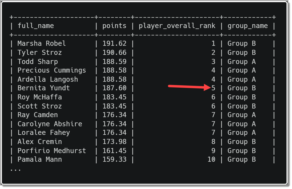
If we decided not to skip numbers when two values are the same, we would use DENSE_RANK() as in the query below.
SELECT `full_name`,
       `points`,
       DENSE_RANK() OVER(
          ORDER BY `points` desc
          ) player_overall_rank,
       `group_name`
FROM `player`
ORDER BY player_overall_rank;
The image below shows the results of using DENSE_RANK(). Note that Bernita Yundt has a ranking of 5 rather than 6 as in the first example.
Using PARTITION BY
While it is interesting to see where each player is ranked compared to everyone else, it does not make it easy to see how players rank within each of the two groups. If we want to show where players rank within their group, we need to use the PARTITION BY clause of our OVER() clause. A partition tells the window function how to group the data into different sets. PARTITION BY works similarly to the GROUP BY clause.
Here is how we would use PARTITION BY to show the rank of each player in their group:
SELECT `full_name`,
       `points`,
       RANK() OVER(
          ORDER BY `points` desc
          ) player_overall_rank,
       `group_name`,
       RANK() OVER( PARTITION BY `group_name`
          ORDER BY `points` desc
          ) player_group_rank
FROM `player`
ORDER BY group_name, player_group_rank;
Note that we added another column, player_group_rank, to the result set that uses a PARTITION BY clause, and we are using group_name as the partition. The partition will tell MySQL to restart the ranking when the group changes. If you do not provide a partition, MySQL will treat the entire results set as a single partition. This partition definition is how we got the rankings of each player across both groups. Note that in the ORDER BY clause, we first sort by the group name and then the ranking within that group.
Here are the results of this query:
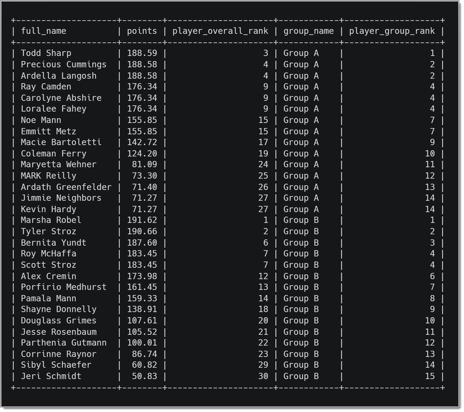
We can see now that each player is listed in their group sorted by their ranking within that group. While Todd Sharp is the 3rd ranked player overall, he is the highest-ranked player in Group A. We can also see that while Ray Camden is 9th overall, he is in a tie for 4th in Group A.
FIRST_VALUE() Example
We now have a helpful ranking of each player within their group. However, what if we wanted to show how many points a player is from being ranked 1st in their group? We can accomplish this by using a window function named FIRST_VALUE(). As you may have guessed by its name, FIRST_VALUE() will return the data value from the first row in a partition. It differs slightly from what we have seen already in that we pass in the column name for the value we wish to return.
Here is the query to return how many points out of 1st place a player is for their given group.
SELECT `full_name`,
      `points`,
      `group_name` group_name,
      RANK() OVER(
      PARTITION BY `group_name`
      ORDER BY `points` desc
      ) player_group_rank,

        points - FIRST_VALUE( points ) OVER (
            PARTITION BY `group_name`
            ORDER BY points DESC
        ) points_back_of_first

FROM `player`
ORDER BY group_name, player_group_rank;
By passing in the argument, points, to FIRST_VALUE(), we retrieve the value of the points column from the first row in the partition. To calculate how many points back from 1st place a player is, we need to do something different than what we have done so far. We need to subtract the points of the partition’s first row from the player’s points in the current row. In this example, we use the result of our call to FIRST_VALUE() in an equation. To me, this is one of the cool things about window functions, and we are not limited to simply adding the results of the function call to a result set. We can use them like we can any other value – including using the values in a WHERE clause or as part of a CASE statement (we will see an example of the latter shortly).
The result of this query looks like this.
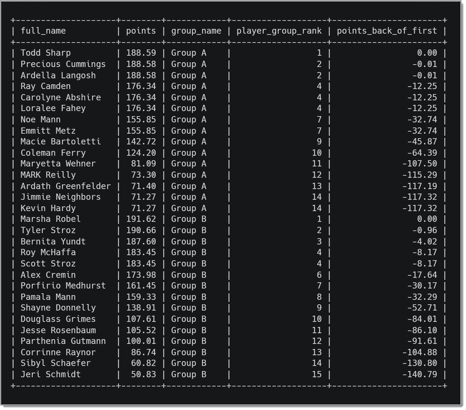
When we view these rankings, it is much easier to determine how far back a player is from the player ranked 1st. It would be trivial to handle this programmatically in any programming language. Returning this data as part of the result set makes it a more straightforward process by returning this data in the result set.
NTH_VALUE() Example
Our fictional competition has playoffs at the end of the regular season. The top 4 teams in each group advance to the playoffs. While it is nice to see how many points a player is out of 1st place, it might be more beneficial for players to see how many points they are from clinching a playoff spot. We use the NTH_VALUE() window function to accomplish this.
SELECT `full_name`,
       `points`,
       RANK() OVER( PARTITION BY `group_name`
          ORDER BY `points` desc
          ) player_group_rank,
       points - FIRST_VALUE( points ) OVER (
          PARTITION BY `group_name`
          ORDER BY points DESC
          ) points_back_of_first,
       CASE
         WHEN NTH_VALUE( points, 4 ) OVER(
            PARTITION BY `group_name`
            ORDER BY points DESC
            ) IS NULL THEN 0
         ELSE points - NTH_VALUE( points, 4 ) OVER(
            PARTITION BY `group_name`
            ORDER BY points DESC
         )
      END AS points_from_playoffs
FROM `player`
ORDER BY group_name, player_group_rank;
Here is the example of using window functions in a CASE statement I promised.
Let’s first look at how we use NTH_VALUE() and then talk about how we use it in the CASE statement. As you can see, we use two arguments for NTH_VALUE(). The first is the column we wish to use, as, in the previous example, we are using the value of the points column. The second argument is the row number in the result we want to look at. In our example, we want to compare every row with the value in the 4th row, so we pass in a value of 4. So, in a nutshell, our call to NTH_VALUE() tells MySQL to retrieve the value of the points column in the 4th row of the partition.
You may be wondering why we decided to use a CASE statement for this value, and the simple answer is for consistency. In this situation, we use the CASE to ensure that we always return a number in the result set. As you can tell by the WHEN in the CASE statement, sometimes, window functions will return NULL. In this instance, the first three rows would return NULL because the 4th row does not yet exist for us to make the comparison. The CASE statement ensures that if the value returned from NTH_VALUE() is NULL, we return the value of 0 (because the players ranked 1 through 3 are still 0 points from having a playoff spot). If the value returned from NTH_VALUE() is not null, we subtract that value from the points value for the current row and return the result.
Here is the result of the above query:
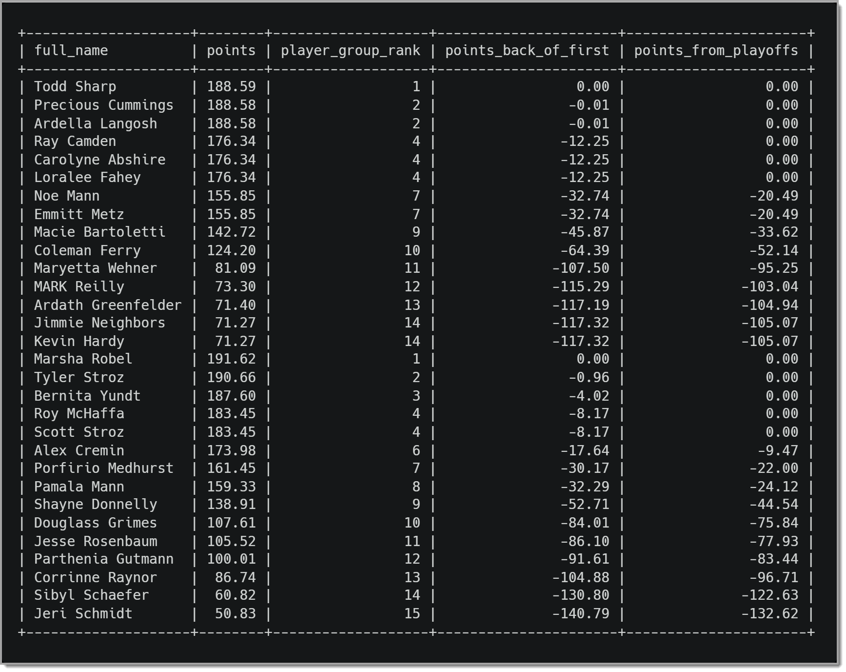
It may seem strange that more than four teams are 0 points from a playoff spot for each group. For example, in Group A, we have two teams tied for 2nd place and three in a tie for 4th place. In Group B, we have two teams tied for 4th place. If we had teams tied at the end of the season, we would need to use a tiebreaker to determine who would make the playoffs. Depending on the tiebreaker rules, we could add that logic to the query to ensure the teams tied in points are displayed based on the tiebreaker information.
Wrap-up
As we have seen, window functions offer us a variety of ways to return data related to other rows in the data set. We discussed the basic syntax for window functions and showed examples of using non-aggregate window functions in our result set.
Hopefully, you better understand the syntax of MySQL window functions.
In the next post, we will explore other window functions and expand our understanding of the different parts of the OVER() clause.
If you want to learn more about Window Functions in MySQL, head over to the documentation.
Photo by Amel Majanovic on Unsplash
